Introduction to Maximum Likelihood Estimation
Introduction
In the previous two posts
we explored the derivation of a univariate OLS regression
graphically and with some simple algebra
and then extended the derivation to account for multiple predictors with
matrix form derivation.
In this post we'll introduce the maximum likelihood estimation with a very simple problem
to understand the role of likelihood in regression problems in subsequent posts.
A blog about probabilities would be dull without a coin toss example. So here it comes:
Intuition Behind Maximum Likelihood Estimation
Let's begin with a dataset of five coin tosses. Four of the tosses landed heads and one of them landed tails, i.e. 5 tosses, 4 heads and 1 tails.
| toss number | Heads | Tails |
|---|---|---|
| 1 | 1 | 0 |
| 2 | 1 | 0 |
| 3 | 0 | 1 |
| 4 | 1 | 0 |
| 5 | 1 | 0 |
Now we can calculate the probability for this outcome for a fair coin.
Let's denote the number of tosses as n, number of heads as k and the probability of heads as theta.
For a single permutation the probability can be obtained by calculating:
\[\theta^{k} * (1-\theta)^{n-k} \\
=0.5^{4} * 0.5^{5-4} \\
=0.5^5 \\
=0.03125
\]
So there's around 0.03125 change that we would get this permutation (the order of heads: 1, 1, 0, 1, 1)
with a fair coin and five tosses.
But we are not interested in this permutation, but the number of heads. Thus, we account
for other permutations as well to calculate the probability of 4 heads.
There are five possible permutations for 5 tosses and 4 heads. In the matrix below columns correspond to
series of tosses - 1 represents a head, whereas 0 represents a tail:
\[\begin{bmatrix}
1 & 1 & 1 & 1 & 0\\
1 & 1 & 1 & 0 & 1\\
1 & 1 & 0 & 1 & 1\\
1 & 0 & 1 & 1 & 1\\
0 & 1 & 1 & 1 & 1\\
\end{bmatrix}
\]
As we know the probability of one permutation and the permutations are equally likely,
we could just multiply the earlier probability of one permutation by 5, but we can
introduce the binomial coefficient just for the heck of it. The binomial coefficient
makes sure that with n trials and k successes, we account for each permutation.
\[\dfrac{n!}{k!(n-k)!} * \theta^{k} * (1-\theta)^{n-k} \\
=\dfrac{5!}{4!(5-4)!} * 0.5^{4} * 0.5^{5-4} \\
=\dfrac{120}{24} * 0.5^5 \\
=5 * 0.03125 \\
=0.15625
\]
The probability of 4 heads of five tosses for a fair coin is around 0.15.
So far we have assumed that our coin is a fair one, but what if it is not.
Then we could estimate the coin bias with maximum likelihood estimation. The question is:
What is the most likely value for the coin bias (the probability of heads)
given the data that we have observed?
We have laid the ground work for maximum likelihood estimation in the earlier calculation when we calculated
the probability of 4 heads out of 5 tosses with a coin that generates heads
with 0.5 probability. Let's calculate the probability of 4 heads out of 5 tosses for nine different hypothetical coins
that generate heads with varying probabilities: 0.1, 0.2, 0.3, 0.4, 0.5. 0.6, 0.7, 0.8, 0.9.
\[\dfrac{n!}{k!(n-k)!} * \theta^{k} * \theta^{n-k} \\
p(k=4, n=5|\theta=0.1) = 5 * 0.1^{4} * 0.9^{5-4} = 0.00045 \\
p(k=4, n=5|\theta=0.2) = 5 * 0.2^{4} * 0.8^{5-4} = 0.0064 \\
p(k=4, n=5|\theta=0.3) = 5 * 0.3^{4} * 0.7^{5-4} = 0.02835 \\
p(k=4, n=5|\theta=0.4) = 5 * 0.4^{4} * 0.6^{5-4} = 0.0768 \\
p(k=4, n=5|\theta=0.5) = 5 * 0.5^{4} * 0.5^{5-4} = 0.015625 \\
p(k=4, n=5|\theta=0.6) = 5 * 0.6^{4} * 0.4^{5-4} = 0.2592 \\
p(k=4, n=5|\theta=0.7) = 5 * 0.7^{4} * 0.3^{5-4} = 0.36015 \\
p(k=4, n=5|\theta=0.8) = 5 * 0.8^{4} * 0.2^{5-4} = 0.4096 \\
p(k=4, n=5|\theta=0.9) = 5 * 0.9^{4} * 0.1^{5-4} = 0.32805 \\
\]
You might notice that the probabilies do not sum up to one. That's not supposed to happen as these are
conditional probabilities from different distributions as the parameters vary.
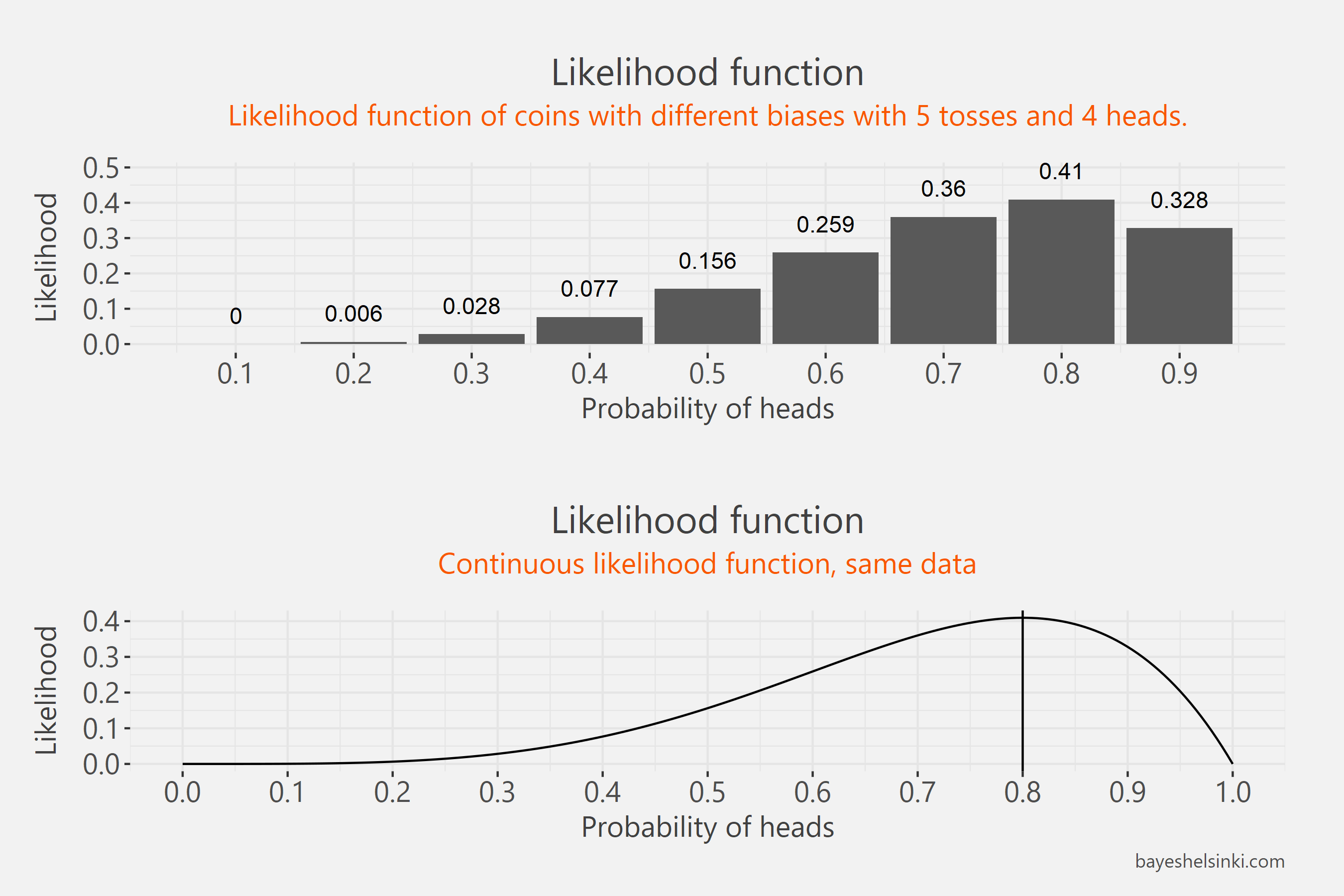
If we plot these values we can outline the likelihood function.

In the figure the same likelihood function is plotted twice - first by plotting only the values we calculated above
and next by varying the probability of heads continuously.
We can see that the value maximizes at 0.8. This is our maximum likelihood estimate of the coin bias -
the probability of heads.
This would have not required much math at all, since the maximum likelihood estimate in this simple case is just
the proportion of heads we have obtained - 4 out of 5.
The likelihood function is not a proper probability function. The values are probabilies, but they are not
probabilities from the same distribution, but from different distributions.
With a probability distribution we are varying the data and keeping the
parameters fixed - with likelihood the data are fixed and the parameters are varying.
This is why we do not use the probability notation with likelihoods:
\(
p(x|\theta)
\)
. This statement tells the probability of some data (e.g. a number of heads, x denotes data)
given some parameter value for the distribution (e.g. the coin bias). The probability distribution is a function of data conditional on
parameter values and it yields probabilities.
With likelihoods we denote:
\(
\mathcal{L}(\theta|x)
\)
. This statement is a function parameters conditional on data and yields likelihood values (probablities from multiple
probability distribution while keeping the data fixed).
The table below illustrates
the different probability functions and the likelihood function.
Each of the columns represents a binomial probability distribution with 5 tosses
\(
p(x|\theta)
\)
. Note how the probabilities of different outcomes
sum up to one. The likelihood function
\(
\mathcal{L}(\theta|x)
\)
is the cross-section of multiple probability distributions with the same data.

The maximum likelihood estimate is the highest value of the cross-section of multiple distributions with different
parameters. The distribution with highest conditional probability is most likely to have generated the data -
a coin that returns heads 80 % of the time is most
likely to have generated our data: 4 heads out of 5 tosses.
The parameter of this distribution is our maximum likelihood estimate.
The table above actually visualizes five different likelihood functions - each row of the table is a separate
likelihood function with identical functional form, but conditional on different data. Note how the maximum value of each row corresponds to
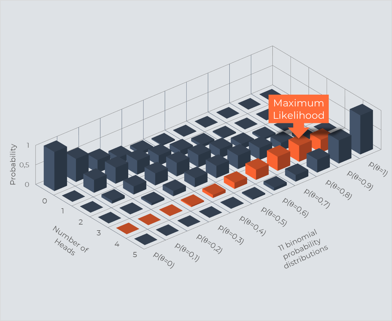
the proportion of heads of that data. Finally, to be a little gimmicky, we can plot the same table as a 3d plot.
The orange columns come from 11 different binomial distributions and we can see that the maximum value is reached at 0,8.

Derivation of Maximum Likelihood Estimate for a Bernoulli distribution
Hopefully, the reasoning above gave you the intuition behind MLE. As with the OLS estimation
we explored first the graphical aspect and then the algebra. We'll proceed here likewise.
To recap, remember that the maximum likelihood method solves the maximum value
of the likelihood function.
We'll use the bernoulli distribution to estimate the most likely parameter. The Bernoulli distribution is a special
case of the binomial distribution when the number of tosses is 1.
Bernoulli distribution and binomial distribution will yield the same
estimate for a coin bias as the binomial distribution just accounts for multiple permumations with same number of heads.
The bernoulli distribution is the following:
\[
p(x|\theta)=\theta^{x}(1-\theta)^{1-x}
\]
In which, theta is the parameter of interest, the coin bias.
x denotes the coin flip outcome: 1 if the coin lands heads and 0 if tails.
The bernoulli distribution itself handles only single tosses and to account for multiple tosses,
we have to multiply the bernoulli distribution by itself n times.
\[
\mathcal{L}(\theta)=\prod_{i=1}^n \theta^{x_i}(1-\theta)^{1-x_i}
\]
This is our likelihood function that we are trying to maximize.
The above uses the product operator and is equal to:
\[=\theta^{x_1}(1-\theta)^{1-x_1} * \\
\theta^{x_2}(1-\theta)^{1-x_2} * \\
... * \\
\theta^{x_{n-1}}(1-\theta)^{1-x_{n-1}} * \\
\theta^{x_n}(1-\theta)^{1-x_n}
\]
We could continue with the product form and derive the ML parameter esimate with that, but at this point
it is useful to take a logarithm of the statement. The reason to use logarithms is to make the calculation
easier - it is much more simple to deal with sums than products. Another reason, which is a more important one,
is that all of the values that are being multiplied in the statement are below zero. If you'll have a large
amount of data and you'd like to estimate the parameter value, you'll quickly bumb into an underflow problem as the
outcome becomes too small for the CPU or memory to handle and you'll end up with a value of zero - try raising a value
of 0.1 in Excel to the millionth power and check if the result is equal to zero.
By using the product rule of logarithms we obtain:
\[=log(
\theta^{x_1}(1-\theta)^{1-x_1} * \\
\theta^{x_2}(1-\theta)^{1-x_2} * \\
... * \\
\theta^{x_{n-1}}(1-\theta)^{1-x_{n-1}} * \\
\theta^{x_n}(1-\theta)^{1-x_n})\]
\[=log(\theta^{x_1}(1-\theta)^{1-x_1}) + \\
log(\theta^{x_2}(1-\theta)^{1-x_2}) + \\
... + \\
log(\theta^{x_{n-1}}(1-\theta)^{1-x_{n-1}}) + \\
log(\theta^{x_n}(1-\theta)^{1-x_n}))\]
\[=\Sigma_{i=1}^n log(\theta^{x_i}(1-\theta)^{1-i})
\]
Next we use the product rule again and the power rule to turn the exponents to multipliers:
\[
\mathcal{L}(\theta)=\Sigma_{i=1}^n (x_i log \theta + (1-x_i)log(1-\theta)) \\
\]
As we are looking to solve for the maximum value of the likelihood function and the parameter value that maximizes it, we have a maximization problem:
\[
\underset{\theta}{arg\,max} \mathcal{L}(\theta)\\
\]
To find the maximum value, we differentiate with the respect to theta and find the root. If this is unclear,
lookup differentation rules for logarithms.
\[
\frac{\delta}{\delta\theta}\mathcal{L}(\theta)=0 \\
\Sigma_{i=1}^n (x_i \frac{1}{\theta}) + \Sigma_{i=1}^n ((1-x_i)\frac{1}{1-\theta}(-1)) = 0\\
\frac{1}{\theta}\Sigma_{i=1}^n( x_i ) + \frac{1}{1-\theta}\Sigma_{i=1}^n (-1+x_i) = 0\\
\frac{1}{\theta}\Sigma_{i=1}^n (x_i) + \frac{1}{1-\theta}\Sigma_{i=1}^n (x_i)
+ \frac{1}{1-\theta}\Sigma_{i=1}^n(-1)= 0\\
\Sigma_{i=1}^n (x_i)(\frac{1}{\theta} + \frac{1}{1-\theta})
+ \frac{1}{1-\theta}(-n)= 0\\
\Sigma_{i=1}^n (x_i)\frac{1}{\theta(1-\theta)}
- \frac{n}{1-\theta} = 0\\
\Sigma_{i=1}^n (x_i)\frac{1}{\theta} - n = 0\\
\Sigma_{i=1}^n (x_i)\frac{1}{\theta} = n\\
\Sigma_{i=1}^n (x_i) = \theta n\\
\hat{\theta} = \frac{\Sigma_{i=1}^n x_i}{n}\\
\]
As you can see the maximum value of the likelihood function for the parameter equals the proportion of successes in
the data. For our coin toss example:
\[
\hat{\theta} = \frac{\Sigma_{i=1}^n x_i}{n}\\
\hat{\theta} = \frac{1+1+0+1+1}{5} = 0.8\\
\]
The result might seem a bit unsatisfactory as we did a lengthy calculation just to prove that the most likely value
for the coin bias is just the proportion of heads in the observed data.
However, the above principles are the same as with more complex maximum likelihood estimations. In the next
post we'll cover the maximum likelihood estimation for a normal distribution and then we'll extend the model
for a regression framework.