
Graphical Intuition of OLS Estimation
Introduction
This is the first in series of blog posts that introduces various
aspects of regression modeling:
ordinary least squares estimation of single variable regression and with multiple variables,
maximum likelihood estimation and finally bayesian regression with a complete for dummies
approach.
These first blog posts are meant to ease the efforts of those just
beginning their path of statistical modeling or for those that want to gain intuitive
understanding of the topic.
Here we go!
Graphical Derivation of Simple Linear Regression Coefficients
Let's begin with some artificial data: A very basic example could be that we have gathered measurements of weights and heights of five people and want to find out the relationship between these two variables - namely we want to find out: can we explain weights of people with the corresponding heights. The table below illustrates these measurements - heights in cm and weights in kilograms.
| name | weight | height |
|---|---|---|
| Matt | 65.0 | 160.0 |
| Donald | 75.0 | 162.5 |
| Tom | 70.0 | 165.0 |
| Dick | 75.0 | 170.0 |
| Harry | 82.5 | 172.0 |
Let's begin by examining this relationship with a scatter plot.
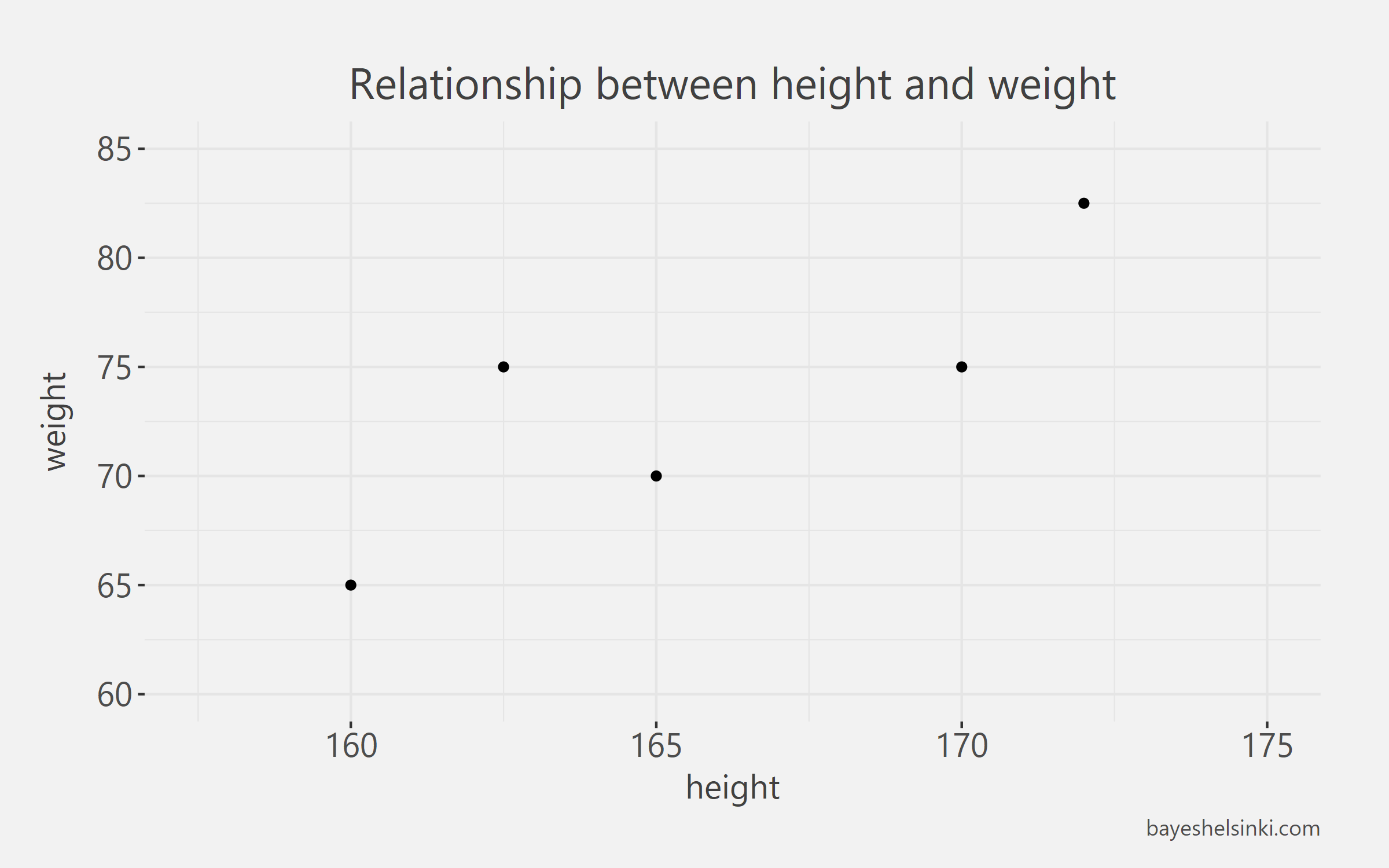
Now as we are interested in linear regression modeling, we would like to find out How much on average does weight increase as we increase height?
Note that we are not saying anything about causality here - we do not claim that height causes more weight. We are just constructing a model, which turns heights into predicted weights, to illustrate how the ordinary least squares estimation works.
Eyeballing the original scatter plot you can see that on average it would seem that weight increases with height (duh, now this is science!), potentially linearly. The OLS regression approximates the mean weights conditional on height. What does this mean? It means that for each value on the x-axis (height), we get an expected value of y, weight \(y=E(y|x)\). The interpretation works if the errors made by our model are evenly spread around the regression line. To ease our graphical derivation, let's take for granted the property that the regression line passes through the point: mean of weights and the mean of heights (illustrated with an orange dot in the graph). Every OLS regression line will satisfy this property. Now let's draw an increasing line through this point so that there will be approximately at least error to the actual data points as possible:
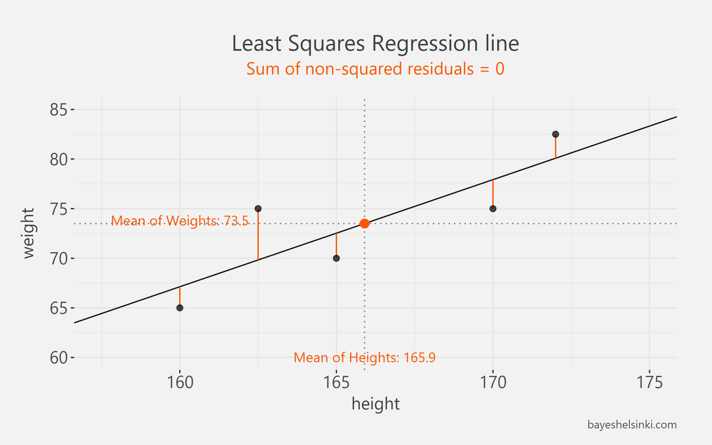
Looks like we did a pretty good job with our approximate line. This line has a simple equation \[\widehat{weight_i} = \beta_0+\beta_1*height_i\] which states that each weight can be approximated with height - the hat above weight denotes that any weight given by our model is an estimate. The parameters \(\beta_0\) (intercept) and \(\beta_1\) (slope) are the unknown parameters we are trying to find out. The value of \(\beta_1\) describes how much we expect the weight to change as we increase height by one centimeter.
We can see that for each of the five weights our model makes a mistake, depicted with orange deviations from the line. To clarify the distinction between \(\widehat{weight_i}\) and \(weight_i\), it can be noted that each point on the line is an estimate of someone’s weight given that we know his height. Thus, the points on the line are the \(\widehat{weight_i}\) values. The real \(weight_i\) are the observed five weight values, depicted with individual five points. The residual, \(e_i=weight_i-\widehat{weight_i}\), is the difference between each observed value and estimated value.
The increasing line that we drew is a good guess, but we would like find the best line that makes the least error possible to the actual data points, \(weight_i\).
How to find out, which values of intercept and slope parameters would yield us the ideal fit?
First solution that many think of is to find a line that minimizes the sum of the residuals - i.e. the suggestion would be: let’s find some values of slope and intercept so that the sum of residuals would be minimized: \(min(e_{Matt}+e_{Donald}+e_{Tom}+e_{Dick}+e_{Harry})\).
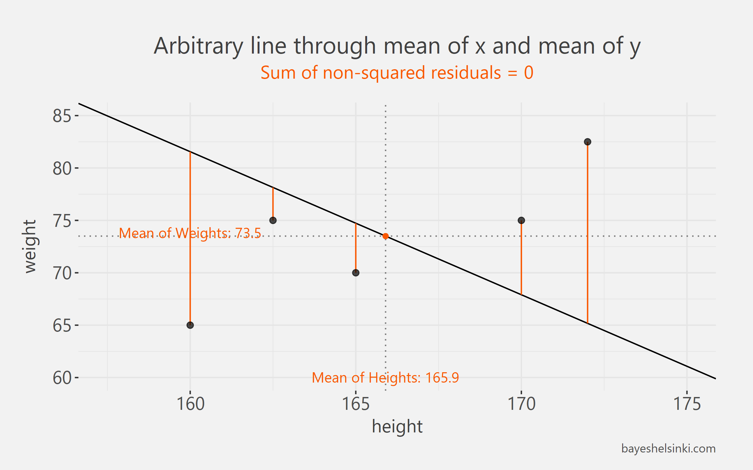
Turns out that this method wouldn’t work too well. Actually, any line that goes through the mean of x and mean of y minimizes the residuals made by the model! This would not be very useful as there are infinite amount of such lines. The chart below illustrates this point. A completely different line passing through the same data and same point of two means, would also minimize the sum of residuals. Sum of residuals in both of these cases would equal to zero. This is because the models make positive and negative errors and as we sum those they cancel each other out and sum to zero: \(\Sigma_i^n e_i = e_{Matt}+e_{Donald}+e_{Tom}+e_{Dick}+e_{Harry}=0\).
We need a method to prevent the positive and negative residuals from canceling each other out and this is exactly what Ordinary Least Squares method does. With OLS we find a line that minimizes the squared residuals made by the model: \(min(e_{Matt}^2+e_{Donald}^2+e_{Tom}^2+e_{Dick}^2+e_{Harry}^2)\).
The best way to understand this minimization is graphically. To illustrate the point of squares, let’s change the aspect ratio of the chart. The OLS regression minimizes the sum of the areas of the squares on the plot - easy, huh?
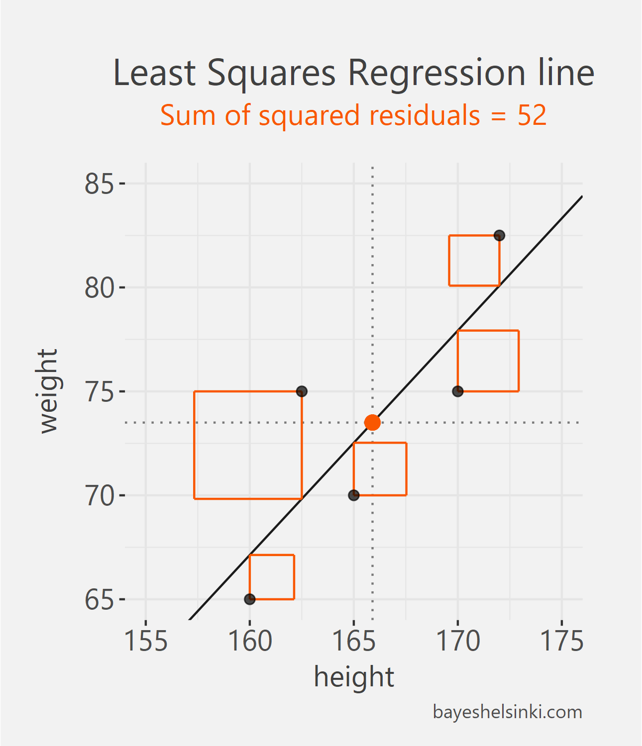
All other lines than the one found with the OLS method would have larger total area of the squares, i.e. larger Sum of Squared Errors, SSE. This can be animated by rotating the line around the mean point of x and y and calculating the total area of the squares for each line with different slopes. In the figure below we have five different arbitrary lines that go through the mean point.
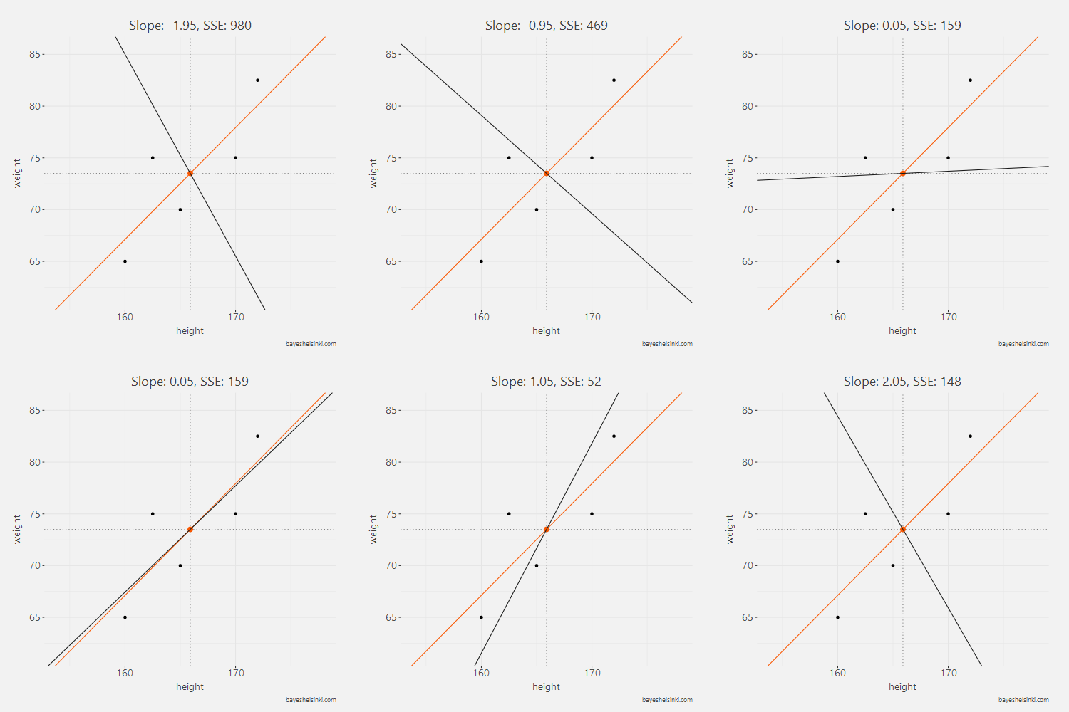
For each line, we calculate the SSE and see that as the slope parameter approaches the OLS line (orange line in graph) from the negative side, the SSE gets smaller. As the line rotates beyond the OLS line, the SSE will begin to increase.
All of the five slope and intercept parameters and their corresponding SSE can be found from the table below.
| Slope | Intercept | SSE |
|---|---|---|
| -1.95 | 397 | 980 |
| -0.95 | 231 | 469 |
| 0.05 | 65 | 159 |
| 1.05 | -101 | 52 |
| 2.05 | -267 | 148 |
Note that none of the five lines here is our OLS line. The OLS parameter value is around 1.08. The above table can be further illustrated by plotting SSE againts the slope parameter. With this exercise, we can see that a parabola function shape is emerging - this is very clear as we think that the SSE is a quadratic function of the residuals and the residuals are directly affected by the slope parameter.
To find a minimum of such parabola, we have to find the point of that parabola that has a slope of zero, i.e. a point in which the SSE will not decrease nor increase. The minimum point of this parabola is the OLS estimate for the slope parameter.
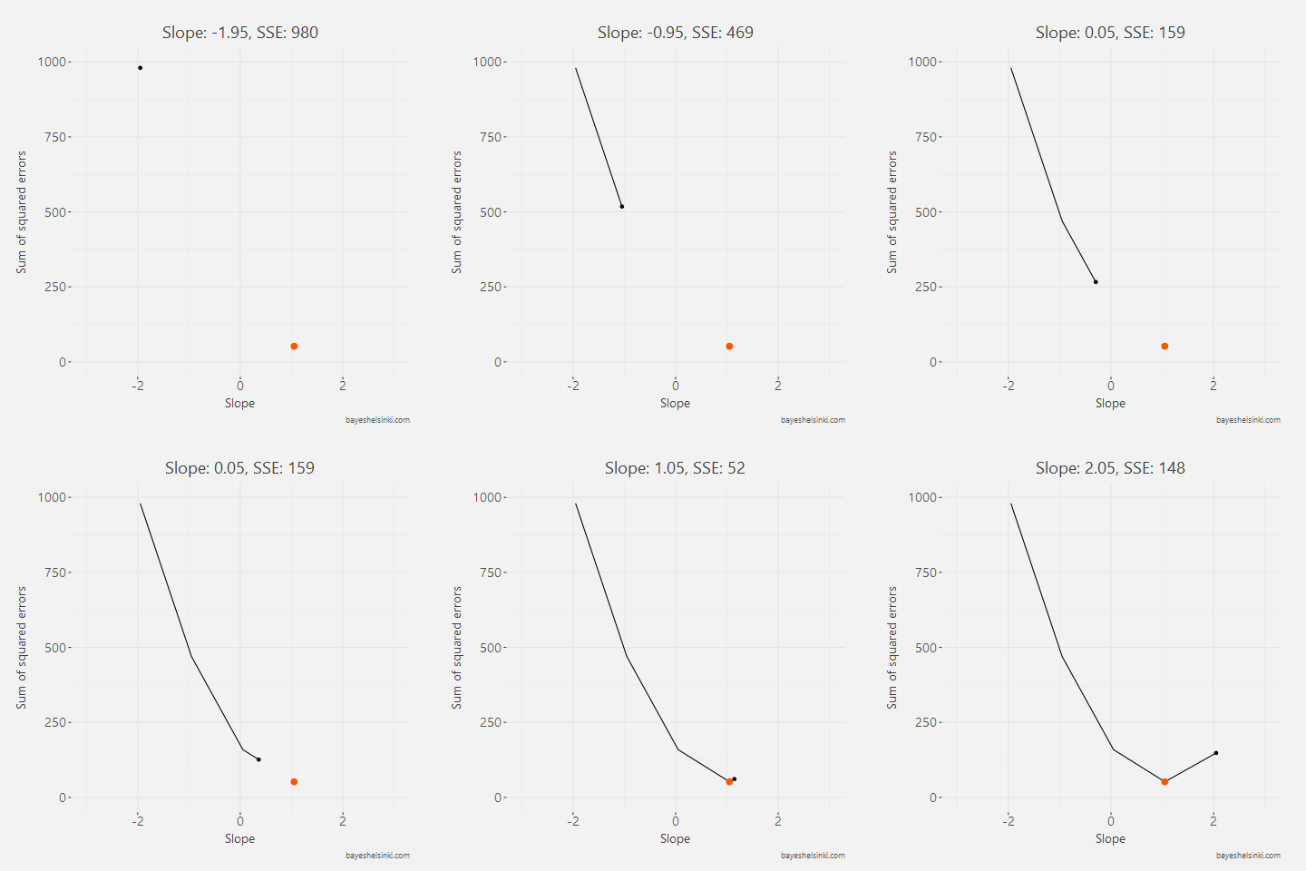
BOOM! There you have it! The graphical derivation makes the OLS very intuitive! Next we’ll proceed to the mathematical derivation to close gap between the algebra and the plots.
The Algebra
As discussed above the equation for a line in x and y space is the following: \[y = \beta_0 + \beta_1 x\] It is very clear that such line could not have generated the observed data as increasing the height, we would just linearly increase the weight and get a straight line. We need some error for the theoretical model to be plausible. Thus, we will add an additional term to account for the noise around the line: \(y = \beta_0 + \beta_1 x + \epsilon\). The noise, \(\epsilon\), are independently and identically distributed random numbers from the normal distribution with zero mean. Note that, above we are not using the subscripts i as we are speaking generally about the theoretical model and not the five observations.
The equation for each of the five different residuals is the following:
\[Residual,e_i = y_i - \beta_0 - \beta_1 x_i\] I have discarded the hat notation in this case for brevity, but to be precise here, each of the beta parameters should have a hat above them. The above equation just states that the residual made by the model for Matt is the real observed value minus the fitted value from our model. \[e_{Matt} =y_{Matt}-\beta_0 - \beta_1 x_{Matt}\]
Now, we would like to find such values for \(\beta_0\) and \(\beta_1\) to make the least amount of error as possible. Consequently, we have ourselves a minimization problem. The graphical derivation illustrated the point that we cannot minimize just the sum of residuals, but we have to minimize the sum of squared residuals. The formula for the squared residuals is: \[e_i^2 = (y_i-\beta_0 - \beta_1 x_i)^2\] and finally the minimization problem is \[min(\Sigma_i^n e_i^2) = min(\Sigma_i^n (y_i - \beta_0 - \beta_1 x_i)^2)\]
The sum or sigma notation \(\Sigma_i^n\), is just a short-hand version of saying \(\Sigma_i e_i^2 = e_1^2+e_2^2+e_3^2+e_4^2+e_5^2\). The subscripts from 1 to 5 denote the five individuals.
Let's open the statement a bit:
\[min(\Sigma_i^n (y_i - \beta_0 - \beta_1 x_i)^2)\] \[=\Sigma_i^n (y_i - \beta_0 - \beta_1 x_i)(y_i - \beta_0 - \beta_1 x_i)\] \[=\Sigma_i^n (y_i^2-2\beta_0y_i+\beta_0^2+2\beta_0\beta_1x_i-2\beta_1x_iy_i+\beta_1^2x_i^2)\]
The above statement is easy to differentiate and then solve for values of slope and intercept. In the next section we solve for intercept.
Derivation of the Intercept Parameter
Next we differentiate with the respect to \(\beta_0\) and \(\beta_1\). Why? Remember that the function above is the sum of squared residuals and this function is the parabola found earlier. The next step is to find the minimum of that parabola and that is done by finding the point where the derivative is zero. Remember that with partial derivatives, we treat other variables as constants. Let’s begin with \(\beta_0\) as it is slightly easier \[\frac{\delta}{\delta\beta_0}\Sigma_i^n (y_i^2-2\beta_0y_i+\beta_0^2+2\beta_0\beta_1x_i-2\beta_1x_iy_i+\beta_1^2x_i^2)\] We get rid of all terms of the polynomial that exclude \(\beta_0\): \[=\Sigma_i^n (-2y_i+2\beta_0+2\beta_1x_i)\] Now let’s set the derivative equal to zero and solve \(\beta_0\). This is called the First Order Condition. \[0=\Sigma_i^n (2\beta_0+2\beta_1x_i-2y_i)\] \[0=\Sigma_i^n (2\beta_0)+\Sigma_i^n(2\beta_1x_i)-\Sigma_i^n(2y_i)\] Next we’ll take the multiplication constants in each summation out of the summation. Remember that if c is constant then \(\Sigma_i^ncx_i = cx_1+...+cx_n=c(x_1+...+x_n)=c\Sigma_i^nx_i\).
\[0=2\Sigma_i^n (\beta_0)+2\beta_1\Sigma_i^n(x_i)-2\Sigma_i^n(y_i)\] Note also that sum of a constant is \(\Sigma_i^nc=nc\). \[0=n2\beta_0+2\beta_1\Sigma_i^n(x_i)-2\Sigma_i^n(y_i)\] Divide both sides by 2. \[0=n\beta_0+\beta_1\Sigma_i^n(x_i)-\Sigma_i^n(y_i)\] Remember that the sum of numbers \(\Sigma_i^nx_i\) divided by the count of numbers \(n\) is the mean \(\bar{x}\). Thus, divide both sides with n and rearrange \(\beta_0\) to LHS.
\[\beta_0=\bar{y}-\beta_1\bar{x}\] Now we have a very simple formula for the intercept parameter - the intercept is just the mean of y minus the mean of x multiplied by the slope parameter.
Derivation of the Slope Parameter
Next, we proceed to derivation of the slope parameter. We’ll begin with the same set up as with the intercept, but this time we’ll differentiate with the respect to slope, \(\beta_1\):
\[\frac{\delta}{\delta\beta_1}\Sigma_i^n (y_i^2-2\beta_0y_i+\beta_0^2+2\beta_0\beta_1x_i-2\beta_1x_iy_i+\beta_1^2x_i^2)\] \[=\Sigma_i^n (2\beta_0x_i+2\beta_1x_i^2-2x_iy_i)\] Set the partial derivative to zero- i.e. the First Order Condition: \[0=\Sigma_i^n (2\beta_0x_i+2\beta_1x_i^2-2x_iy_i)\] \[0=\Sigma_i^n(-2(y_ix_i-\beta_0x_i-\beta_1x_i^2))\] Take the constant out of the summation and divide by -2. \[0=\Sigma_i^n(y_ix_i-\beta_0x_i-\beta_1x_i^2)\] Substitute \(\beta_0\): \[0=\Sigma_i^n(y_ix_i-(\bar{y}-\beta_1\bar{x})x_i-\beta_1x_i^2)\] \[0=\Sigma_i^n(y_ix_i)-\bar{y}\Sigma_i^nx_i+\beta_1\bar{x}\Sigma_i^nx_i-\beta_1\Sigma_i^nx_i^2\] Rearrange terms containg \(\beta_1\) to LHS: \[\beta_1\Sigma_i^nx_i^2-\beta_1\bar{x}\Sigma_i^nx_i=\Sigma_i^n(y_ix_i)-\bar{y}\Sigma_i^nx_i\] Common factor: \[\beta_1(\Sigma_i^nx_i^2-\bar{x}\Sigma_i^nx_i)=\Sigma_i^n(y_ix_i)-\bar{y}\Sigma_i^nx_i\] \[\beta_1=\frac{\Sigma_i^n(y_ix_i)-\bar{y}\Sigma_i^nx_i}{(\Sigma_i^nx_i^2-\bar{x}\Sigma_i^nx_i)}\] Sum of all x equals n times the mean of x: \[\beta_1=\frac{\Sigma_i^n(y_ix_i)-\bar{y}\Sigma_i^nx_i}{\Sigma_i^nx_i^2-n\bar{x}^2}\] This is the trickiest part. Add a zero to the equation \(0=-n\bar{x}\bar{y}+n\bar{x}\bar{y}\): \[\beta_1=\frac{\Sigma_i^n(y_ix_i)-\Sigma_i^n(x_i)\bar{y}-n\bar{x}\bar{y}+n\bar{x}\bar{y}}{\Sigma_i^nx_i^2-n\bar{x}^2}\] Note that \(n\bar{x}\bar{y}\) equals \(\Sigma_i^n(y_i)\bar{x}\), but it also equals \(\Sigma_i^n(\bar{x}\bar{y})\): \[\beta_1=\frac{\Sigma_i^n(y_ix_i)-\Sigma_i^n(x_i)\bar{y}-\Sigma_i^n(y_i)\bar{x}+\Sigma_i^n(\bar{x}\bar{y})}{\Sigma_i^nx_i^2-n\bar{x}^2}\] \[\beta_1=\frac{\Sigma_i^n(y_ix_i-x_i\bar{y}-y_i\bar{x}+\bar{x}\bar{y})}{\Sigma_i^nx_i^2-n\bar{x}^2}\] \[\beta_1=\frac{\Sigma_i^n(y_i(x_i-\bar{y})-\bar{y}(x_i-\bar{x})}{\Sigma_i^nx_i^2-n\bar{x}^2}\] \[\beta_1=\frac{\Sigma_i^n(y_i-\bar{y})(x_i-\bar{x})}{\Sigma_i^n(x_i^2-\bar{x}^2)}\] Wow! There you have it. We could stop here if we wanted to, but now we can easily show another useful property. If we divide both the numerator and denominator by n-1 (these will cancel out, so we won’t break the equation here). We obtain a numerator and a denominator, which we immediately recognize as covariance and variance:
Numerator is the covariance of y and x: \[Covariance=\frac{\Sigma_i^n(y_i-\bar{y})(x_i-\bar{x})}{n-1}\] Denominator is the variance of x: \[Variance=\frac{\Sigma_i^n(x_i^2-\bar{x}^2)}{n-1}\]
Consequently, the slope parameter can also be expressed as
\[\beta_1 = \frac{Cov(x,y)}{Var(x)}\]
This property can be easily verified by calculating covariance of the weights and heights and then dividing the result with the variance of heights. Try it out yourself by running the R code below!
Now we have illustrated the derivation and idea of Simple Linear Regression. To truly master the linear regression (and many other models), we need to solve the same estimators with matrix algebra. This is the topic of the next post.