Maximum Likelihood and Regression
Introduction
So far we have covered maximum likelihood for static parameters. This time we let the mean parameter vary in the model and see how it is equal to a basic regression model.
Moving Normal Distribution
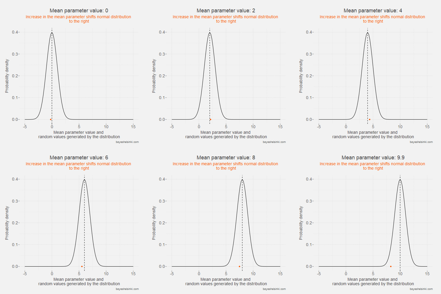
Let's begin by examining visually the kind of data that the normal distribution generates if we increase the \( \mu \) parameter. We keep the standard deviation constant in the following animated model:

The values of the generated data, y, (orange points) increase on average as we increase the mean parameter value (dashed line).
As the standard deviation of the model remains constant as the distribution shifts to the right,
the dispersion of the generated data is on average the same given the mean parameter.
The above animation can be (and was) speficied mathematically:
\[
y \sim N(x, \sigma),
\] that is, y is distributed normally given each x value and constant standard deviation.
The moving normal probability density curve on the other hand is:
\[
p(y|x,\sigma)\\
=\frac{1}{\sigma\sqrt{2\pi}}e^{-\frac{1}{2}(\frac{y-x}{\sigma})^2}
,\]
in which y is vector data points generated by the model and x is a corresponding vector of x values (0, 0.1, 0.2, ... ,10) that shift the model location
along the x-axis and sigma is a constant standard deviation.
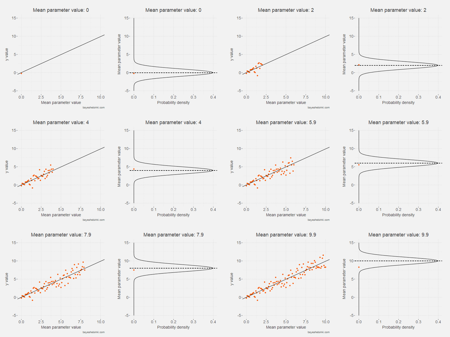
The model can be further illustrated by plotting the generated values on the y-axis and the mean parameter values on the x-axis.
The previous animation is rotated and plotted along the resulting scatter plot.
 Whoa! That looks a lot like a data from a linear regression! That's not a coincidence:
The linear regression model is the same model as specificed here. Recall that as a data generating process (DGP),
the linear regression turns x values into y values with a line equation and then adds random noise around the line equation from
a zero mean normal distribution.
\[
y=\beta_0+\beta_1 x + \epsilon,
\]
in which
\[
\epsilon \sim N(0, \sigma)
\]
Our new moving normal distribution model shifts a normal distribution by varying its mean parameter with given x values
and generates random points, y, around each mean parameter value.
\[
y \sim N(x, \sigma)
\]
Our model is identical to a linear regression model with parameter values
\(
\beta_0=0
\)
and
\(
\beta_1=1
\)
\[
y= x + \epsilon,
\]
Both of our models assume independence and constant variance. In linear regression, the
\(
\epsilon
\) are indenpendent and identically distributed draws from the normal distriubtion and in
our moving normal distribution model the model was specified
as having a constant variance and the draws being independent of each other.
To clarify, it is all the same to generate data from a normal distribution with a mean of, say, 56 and standard deviation of 1
or generate data from the standard normal distribution \(
N(0,1)
\) and then add 56 to each value as is the case with linear regression as a DGP.
Both models produce the same kind of data.
This leads us to specify our moving normal distribution model as a regression model, the \(
\mu
\) parameter is modeled as a line equation \(
\mu = \beta_0+\beta_1x
\) and thus our data generating process becomes:
\[
y \sim N(\mu, \sigma) \\
= y \sim N(\beta_0+\beta_1x, \sigma)
\]
The probability density function for the model is:
\[
p(y|\beta_0, \beta_1, x,\sigma)\\
=\frac{1}{\sigma\sqrt{2\pi}}e^{-\frac{1}{2}(\frac{y-\beta_0+\beta_1x}{\sigma})^2}\]
The joint probability density is:
\[
\prod_{i=1}^n p(y_i|\beta_0, \beta_1, x_i,\sigma)\\
=\prod_{i=1}^n \frac{1}{\sigma\sqrt{2\pi}}e^{-\frac{1}{2}(\frac{y_i-\beta_0+\beta_1x_i}{\sigma})^2}
\] and from here we could easily derive the likelihood function as was done in the previous post.
But we know from previous derivation that the likelihood function for a normal distribution is:
\[
\mathcal{L}(\mu, \sigma)=(\sigma^2 2\pi)^{-n/2} e^{-\frac{1}{2 \sigma^2}\sum_{i=1}^n(y_i-\mu)^2} \\
\]
and we can skip the derivation and just substitute the mu parameter to obtain the linear regression likelihood function:
\[
\mathcal{L}(\beta_0, \beta_1, \sigma)=(\sigma^2 2\pi)^{-n/2} e^{-\frac{1}{2 \sigma^2}\sum_{i=1}^n(y_i-\beta_0+\beta_1x)^2} \\
\]
Even further we can obtain the log-likelihood function with substitution:
\[
=-\frac{n}{2} ln(\sigma^2)-\\
\frac{n}{2} ln(2\pi) - \\
\frac{1}{2 \sigma^2}\sum_{i=1}^n(y_i-\mu)^2 \\
=-\frac{n}{2} ln(\sigma^2)-\\
\frac{n}{2} ln(2\pi) - \\
\frac{1}{2 \sigma^2}\sum_{i=1}^n(y_i-\beta_0+\beta_1x_i)^2 \\
\]
Now, let's experiment with our weight and height data from the first post.
| name | weight | height |
|---|---|---|
| Matt | 65.0 | 160.0 |
| Donald | 75.0 | 162.5 |
| Tom | 70.0 | 165.0 |
| Dick | 75.0 | 170.0 |
| Harry | 82.5 | 172.0 |
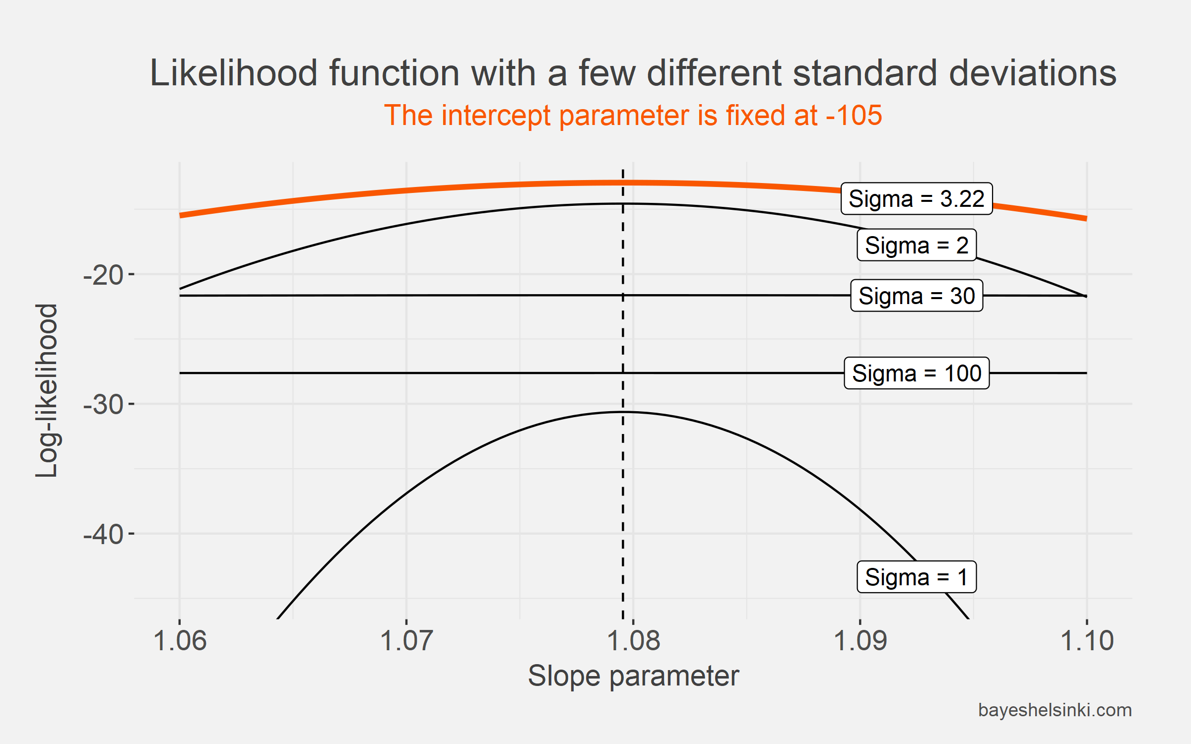
If we plot the log-likelihood function with slope on the x-axis,
we see that the function maximizes, when the slope parameter is at its OLS estimate 1.0795. We also plot several
different curves from the log-likelihood function with different standard deviations and notice that for our selected values
log-likelihood maximizes, when the standard deviation is at 3.22.
We keep the intercept parameter fixed at its OLS estimate for all curves as this makes the plotting easier, but keep in mind that
changing the intercept parameter from the best estimate reduces our likelihood.
 The estimation method is different, but the estimation results are the same for slope and intercept!. This is a special
property: when assuming independence in maximum likelihood and gaussian i.i.d. errors in OLS,
the estimation results coincide.
This begs a question: Why do we go to great lengths to introduce maximum likelihood estimation,
as we could just use the Ordinary Least Squares method?
The first reason is that maximum likelihood is a much more flexible estimation method and allows us to specify a wide range of different
models. The more important reason is that, we are building intuition around the bayesian regression and the likelihood
function is at the core of bayesian estimation. To learn bayesian methods, it is much easier to study first the
frequentist likelihood methods first and then move on to the bayesian paradigm.
In the next post, we derive the maximum likelihood estimators.