
Intuition Behind Maximum Likelihood Estimation of Normal Distribution
Introduction
This time we develop our understanding of maximum likelihood and move from a discrete example to a continuous one. As the ultimate goal of these maximum likelihood posts is to understand the role of maximum likelihood in regression modeling, we'll introduce the continuous problem with normal distribution.
Intuition Behind MLE of Normal Distribution
We'll proceed as with the discrete example from last post, but this time we have continuous data - the heights data from the first post.
| name | height |
|---|---|
| Matt | 160.0 |
| Donald | 162.5 |
| Tom | 165.0 |
| Dick | 170.0 |
| Harry | 172.0 |
We know that adult male heights follow a normal distribution and thus suspect the underlying distribution for our data to be normal.
\[ f(x) = \frac{1}{\sigma\sqrt{2\pi}}e^{-\frac{1}{2}(\frac{x-\mu}{\sigma})^2} \]
Normal distribution has two parameters: mean
\(
\mu
\)
and standard deviation
\(
\sigma
\)
.
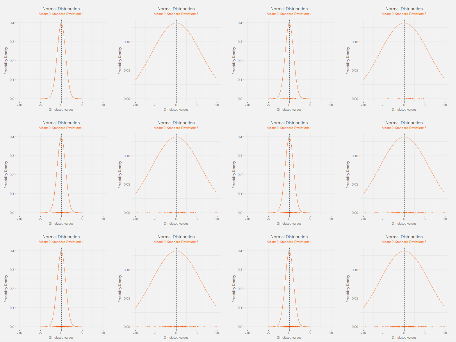
Mean controls the location of the distribution and standard deviation the wideness. We can simulate random
values from the normal distribution to illustrate the kind of data it generates. The two distributions below
have identical means, but different standard deviations. You can see that both distributions generate values
around their means, but the second distribution tends to generate more dispersed values as it has a larger
standard deviation.
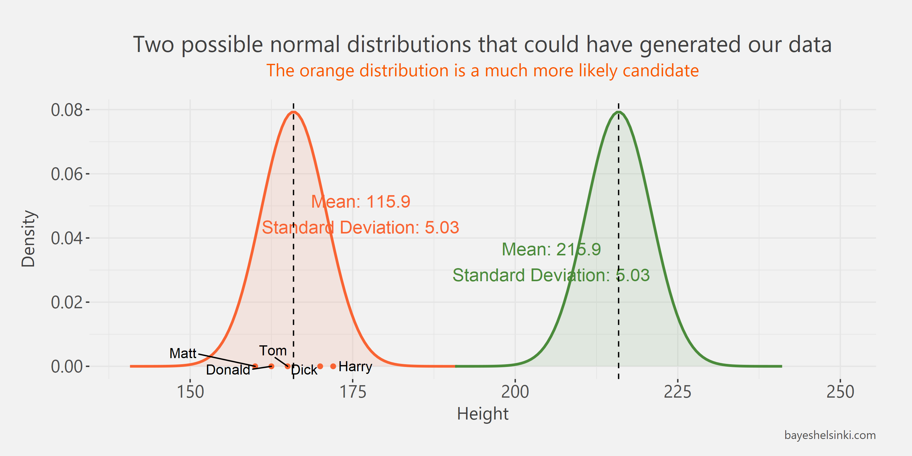
 In the figure below we can see our five data points and two hypothetical normal distributions with different means.
It is clear that our observations are much more likely to have generated from the orange distribution as the
values lay evenly around its mean.
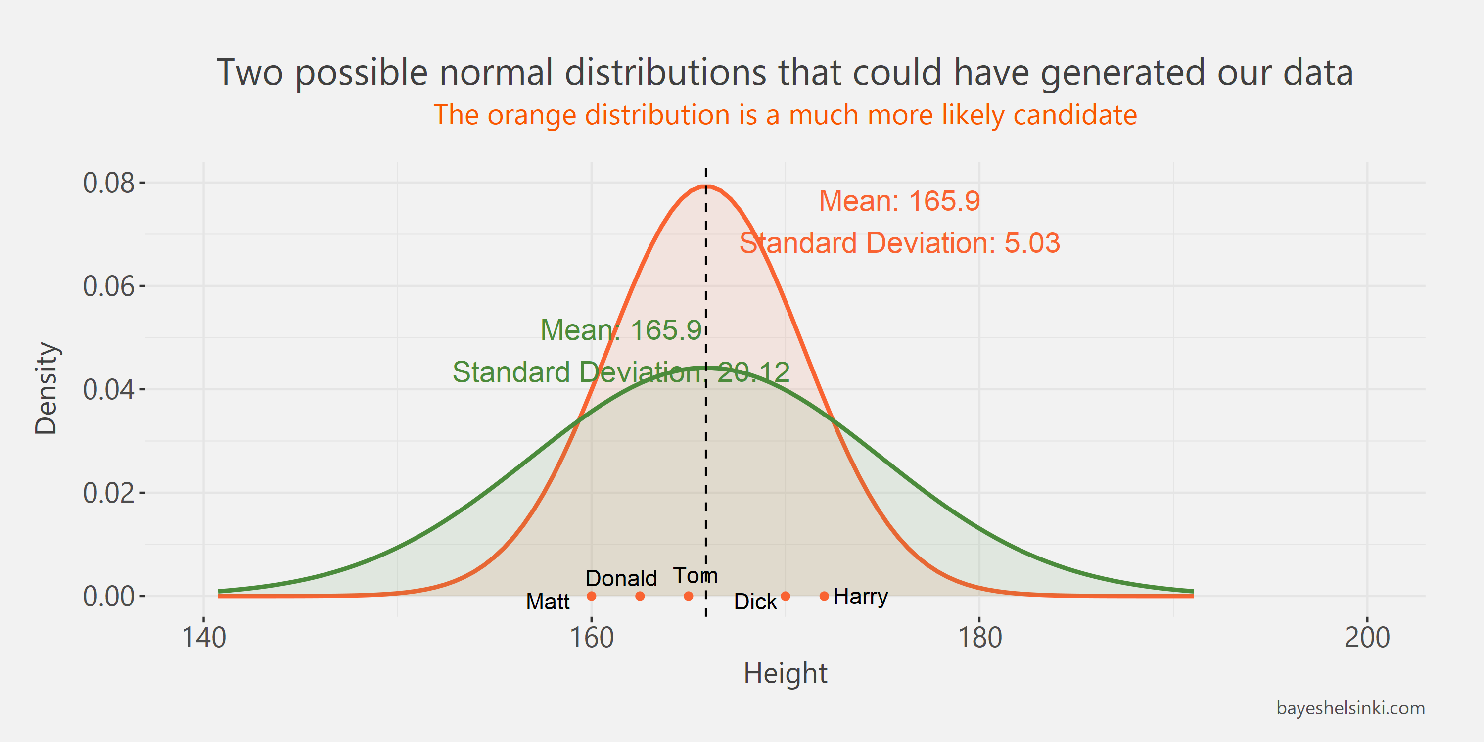
 The next figure has two normal distributions with different standard deviations. Again,
the orange distribution is more likely to generate our observed data than the green distribution - otherwise the values should
be more dispersed around the its mean.
 As with the discrete example from last post, the task for MLE is to find the most likely values for
our distribution. To save you from the anti-climax - those values are the sample mean and sample standard deviation
of our data.
To calculate one data point of our likelihood function, we can decide arbitrary values for our
parameters and calculate the joint probability density of obtaining these data.
Keep in mind that as we have moved to a continuous distribution,
there are infinite amount of outcomes even for five continuous data points - the probability
of obtaining a specific value from a continuous distribution is zero.
Thus, contrary to the coin toss example, the single value of our likelihood function in this example is
not the joint probability of the data given the parameters,
but the joint probability density of the data given the parameters.
If the distinction between probability and probability density is unclear, it is
good to check explanations from Wikipedia.
Remember that the likelihood function varies the parameters
and keeps the observed data fixed, i.e. the values of the likelihood function for some data
come from many normal distributions.
What is the probability density of obtaining the height of Harry, 172, from a normal distribution with
some arbitrary chosen parameter values,
\(
\mu=170
\)
and standard deviation
\(
\sigma=1
\)
? The
\(
p()
\)
notation is used for both probability density and probability.
\[
p(x|\mu,\sigma) = \frac{1}{\sigma\sqrt{2\pi}}e^{-\frac{1}{2}(\frac{x_i-\mu}{\sigma})^2} \\
p(x=172|\mu=170,\sigma=1) = \frac{1}{1*\sqrt{2\pi}}e^{-\frac{1}{2}(\frac{172-170}{1})^2} \\
p(x=172|\mu=170,\sigma=1) = \frac{1}{\sqrt{2\pi}}e^{-\frac{1}{2}(2)^2} \\
p(x=172|\mu=170,\sigma=1) = \frac{1}{\sqrt{2\pi}}e^{-2} \\
p(x=172|\mu=170,\sigma=1) \approx 0.05399 \\
\]
We could also ask what is the probability density of obtaining the height of Dick, 170, (no pun intended)
from the same normal distribution?
Let's shorten the notation for brevity and discard the conditional notation.
\[
p(x=170) = \frac{1}{1*\sqrt{2\pi}}e^{-\frac{1}{2}(\frac{170-170}{1})^2} \\
p(x=170) = \frac{1}{\sqrt{2\pi}}e^{0} \\
p(x=170) = \frac{1}{\sqrt{2\pi}}*1 \\
p(x=170) \approx 0.39894 \\
\]
We can see that the second value is much higher than the first one. As said before, the values 0.399 and 0.054
can not be interpreted as probabilities of obtaining such heights, but they can be interpreted as
relative probabilities of infinitesimally small interval around the values. In other words,
upon sampling a data points from the distribution the values very close to 170 are 7.4
\(
(0.39894 / 0.05399 \approx 7.4)
\)
times more probable to occur than the values around 172.
If the two values are independent of each other, then the joint probability density for the two data points is
the product of the two density values. The assumption of independence is an important one and the estimation
will be different if that assumption does not hold in some problem.
\[
p(x=172, x=170) \\
=p(x=172) * p(x=170) \\
\approx 0.05399 * 0.39894 \\
\approx 0.02154 \\
\]
For the whole dataset of five heights the likelihood for our example parameters, 170 and 1, is:
\[
p(x=160,..., x=172)\\
=p(x=160) * \\
p(x=162.5) * \\
p(x=165) * \\
p(x=170) * \\
p(x=172) \\
\approx 7.694599*10^{-23} * \\
2.434321*10^{-13} * \\
1.486720*10^{-06} * \\
0.39894 * \\
0.05399 \\
\approx 5.998241*10^{-43}
\]
As you can see the likelihood becomes very small very quickly. As explained in the previous blog post,
this would pose a problem with larger datasets and thus we will continue with logarithms.
Now we can do the same thing for our whole dataset.
\[
log(p(x=160,..., x=172)) \\
= log(p(x=160) * \\
p(x=162.5) * \\
p(x=165) * \\
p(x=170) * \\
p(x=172)) \\
= log(p(x=160)) + \\
log(p(x=162.5)) + \\
log(p(x=165)) + \\
log(p(x=170)) + \\
log(p(x=172)) \\
\approx -50.91 -29.04 -13.41 -0.91 -2.91 \\
\approx -97.21
\]
We can replicate the above calculation in the following code snippet, in which we have our data, the heights of five people. We also have our
arbitrary parameters. Run the code without changing it, take note of the resulting log-likelihood
and then try changing the mu and sigma, i.e. mean and standard deviation respectively, and
see how the value of log-likelihood changes. If you change the mu and sigma to sample mean and standard deviation you'll obtain the maximum of log likelihood.
With the coin toss example we varied the value of the coin bias parameter and made a plot of the
likelihood function for our data. We will do the same here, but as the normal distribution has two parameters,
we plot the log-likelihood on the y-axis, the mean parameter on the x-axis and standard deviation as animation.
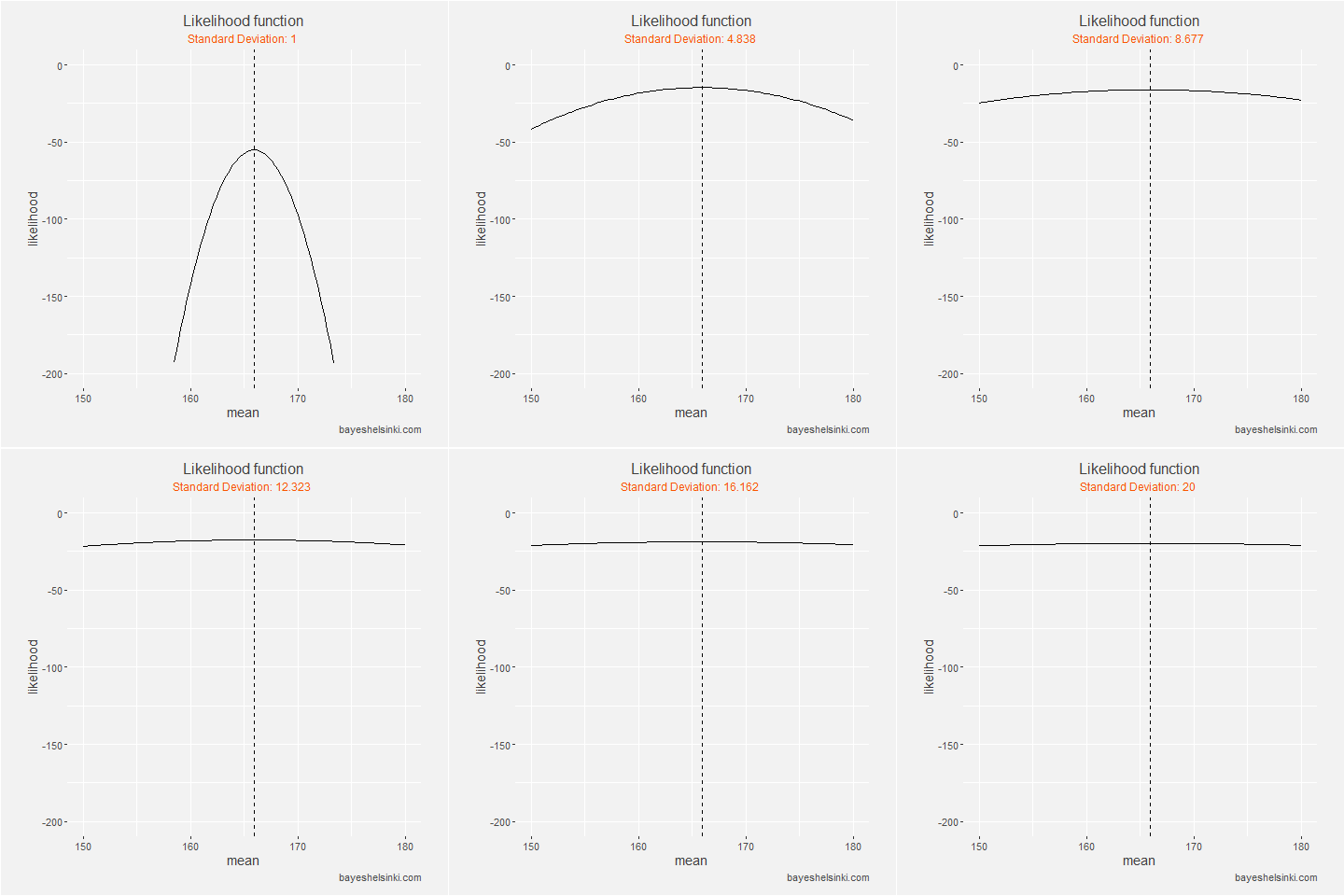 We can see that with the likelihood function is always at it maximum on the dashed line, which is drawn at
sample mean. On the animation axis, the likelihood increases as we increase the standard deviation,
but after it reaches the sample standard deviation of the data, it begins to decrease.
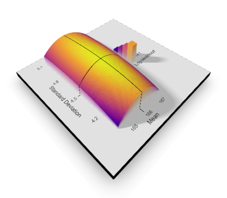
To be even more fancy and again gimmicky, we can plot the likelihood function in 3D with the value of mean on x-axis,
standard deviation on y-axis and log-likelihood on vertical axis.
As you can see the likelihood function is a concave "mountain" that has its highest point at sample mean and standard deviation.
 There you have it! This is the intuition behind maximum likelihood estimation. In the next post, we'll cover the algebra for the derivation.